Species Distribution Modelling

Progress October 2020

Kim Kenobi

Statistics Researcher on species distribution modelling, Aberystwyth University

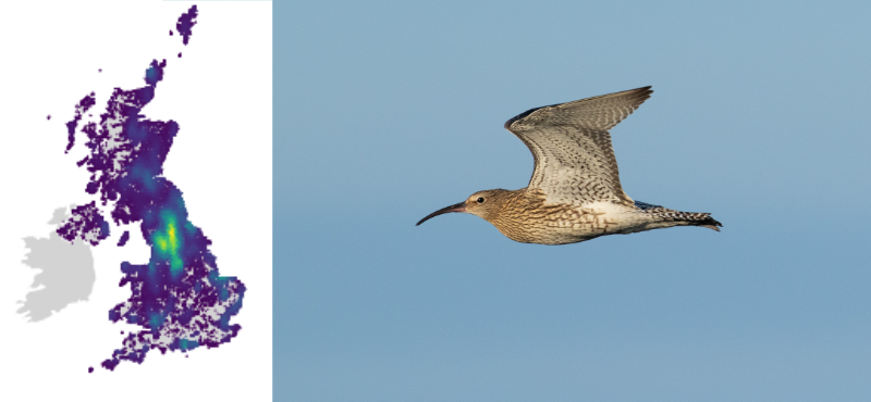
The initial focus of Work Package 3 (WP3) is to consider species distribution modelling for Curlew and Greenland White-fronted Geese at the broad scale of the whole of the UK and Ireland. An important aspect of the work for WP3 in this initial period of the ECHOES project has been to establish what data sources are available in terms of bird observations for each of the two species of interest across the British Isles. 

There are a range of collections of bird observation data, including National Biodiversity Network (NBN) in the UK, to which the British Trust for Ornithology (BTO) is one of the key contributors, and, in Ireland, eBird. 

The data in different data sets come in different formats, in particular in terms of the geographical coordinate system (latitude, longitude vs. eastings and northings for example). Part of the work in gathering and assessing the range of data sets available has been to find common coordinate systems and prepare computer code to group the observations into map squares at any desired resolution. 

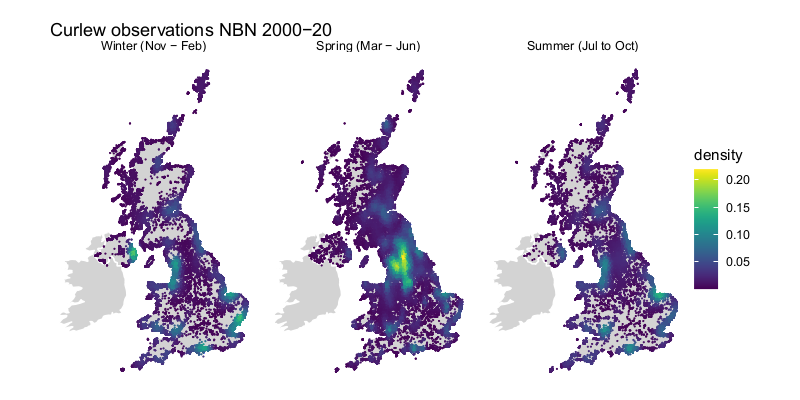
Since we are interested in the wintering grounds of Curlew and Greenland White-fronted geese, we have decided to split the data gathered throughout the year into three periods: November to February (‘winter’), March to June (‘spring’) and July to October (‘summer’).  With this breakdown of data by observation time, we can already begin to see patterns emerging in the data. For example, in Figure 1 below, we see how the distribution of Curlew sightings varies over these three periods of the year for the period 2000–2020 in the NBN data set. 

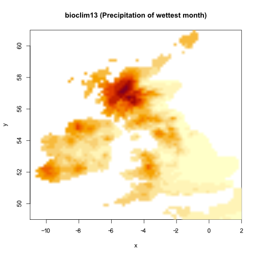
What we have just started implementing in WP3 is using various maps (which we can think of as regular grids with one number per grid cell corresponding to the value of the variable in that grid cell, for example mean annual temperature) as explanatory variables in species distribution modelling. The sorts of questions this line of research will enable us to answer include the extent to which a particular variable (such as for example land cover coded as a set of distinct classes including estuary, mudflats, farmland and so on) can explain the observed variability in the patterns of distribution of curlew and Greenland White-fronted Geese. Just to give an indication of the sorts of maps we might be interested in, we include a coarse-scale map of the bioclim13 (precipitation of wettest month) variable from the Worldclim version 2.0 set of climatic variables. 

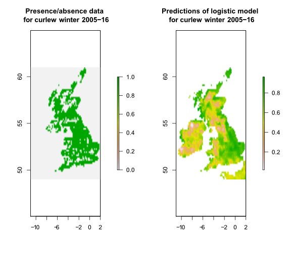
We are only just starting on the species distribution modelling for the bird species. To offer some flavour of where we are heading, consider Figure 3, where we plot the presence/absence of curlew in winter months 2005–16 across grid squares for the British Isles (left hand plot), and the predicted probabilities of seeing Curlew based on a logistic (presence/absence) model that includes four bioclim variables (right hand plot). It is a rudimentary model at this stage, simply included to indicate how we are progressing.